Homework

brms intro

Load the packages we’ll use today

Code

library(tidyverse) # for tidy style coding
library(brms) # for bayesian models
library(tidybayes) # for many helpful functions used to visualise distributions
library(MetBrewer) # for pretty colours
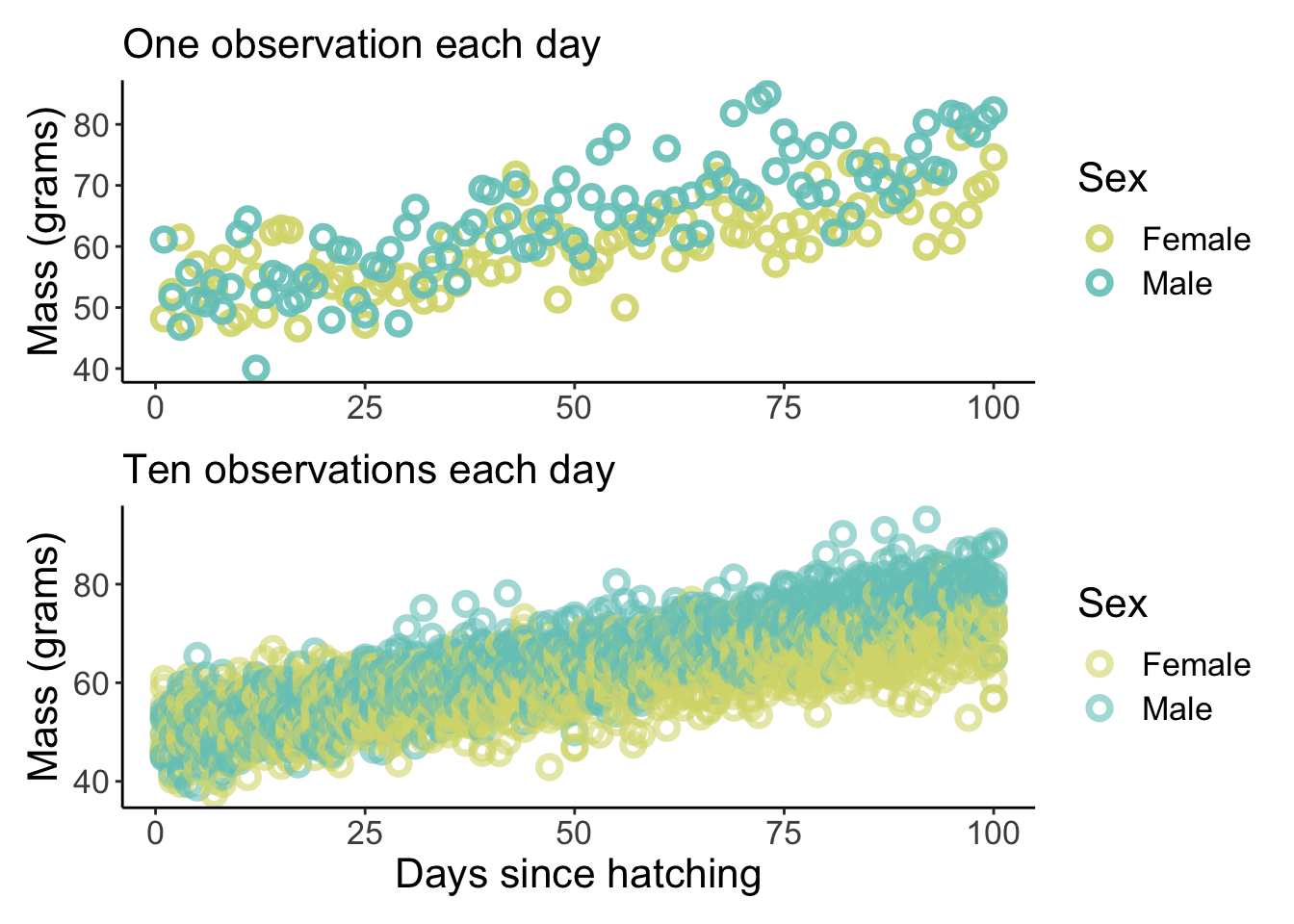
library(patchwork) # for combining plots

Simulating data

Code

sim_growth_data_small <-
  expand_grid(
    Days = rep.int(1:100, 1),
    Sex = c("Female", "Male")) %>% 
  arrange(Sex) %>% 
  mutate(Mass = if_else(Sex == "Female",
                        Days * 0.2 + rnorm(100, 50, 5),
                        Days * 0.3 + rnorm(100, 50, 5)))

sim_growth_data_large <-
  expand_grid(
    Days = rep.int(1:100, 10),
    Sex = c("Female", "Male")) %>% 
  arrange(Days) %>% 
  mutate(Mass = if_else(Sex == "Female",
                        Days * 0.2 + rnorm(1000, 50, 5),
                        Days * 0.3 + rnorm(1000, 50, 5)))

Plot them

Code

p1 <-
  sim_growth_data_small %>%
  ggplot(aes(x = Days)) +
  geom_point(aes(y = Mass, colour = Sex), shape = 1.5, stroke =2, size = 2.5, alpha = 0.9) +
  scale_colour_manual(values = c(met.brewer(name = "Hokusai3")[1], met.brewer(name = "Hokusai3")[3])) +
  labs(x = NULL, y = "Mass (grams)", subtitle = "One observation each day") +
  theme_classic() +
  theme(panel.grid = element_blank(),
        text = element_text(size = 16))

p2 <-
  sim_growth_data_large %>%
  ggplot(aes(x = Days)) +
  geom_point(aes(y = Mass, colour = Sex), shape = 1.5, stroke =2, size = 2.5, alpha = 0.6) +
  scale_colour_manual(values = c(met.brewer(name = "Hokusai3")[1], met.brewer(name = "Hokusai3")[3])) +
  labs(x = "Days since hatching", y = "Mass (grams)", subtitle = "Ten observations each day") +
  theme_classic() +
  theme(panel.grid = element_blank(),
        text = element_text(size = 16))

p1 / p2

Model with brms

The core inputs to make the model run are formula, family and data.

You can code them like this:

brm(Mass ~ 1 + Days, family = gaussian, data = sim_growth_data_small)

Next are your priors

The get_prior function is very useful here. Let’s try it out:

Code

get_prior(Mass ~ 1 + Days, family = gaussian, data = sim_growth_data_small)

                   prior     class coef group resp dpar nlpar lb ub
                  (flat)         b                                 
                  (flat)         b Days                            
 student_t(3, 62.2, 9.6) Intercept                                 
    student_t(3, 0, 9.6)     sigma                             0   
       source
      default
 (vectorized)
      default
      default

This shows the brms defaults for all the priors that are neccessary to run this model. If you don’t supply your own prior, brms will use its defaults.

So we need priors for b, Intercept and sigma

What do thes mean?

• b is the effect that Days has on Mass. We know that things generally get bigger after hatching, so this must be positive.

• Intercept is the value for mass when Days = 0. This also must be positive.

• sigma is the variation in mass. This also must be > 0.

To check out what a prior looks like I use this quick bit of code

Code

hist(rnorm(n = 1000, mean = 0, sd = 1))

Now some modelling nitty gritty

We need to tell brms how many iterations to run the model for, how many of these iterations we wish to use as warmup, how many chains to run and how many of your computers cores you want to use.

Finally, because these models can be slow (this one will be fast but it’s good practice), you can use the file option to save the model output in your working directory and automatically load it whenever you rerun the code.

Here is the full model:

Code

Our_mass_model_small <-
  brm(Mass ~ 1 + Days,
    family = gaussian,
    data = sim_growth_data_small,
    prior = c(prior(normal(50, 10), class = Intercept),
              prior(lognormal(-1, 1), class = b, lb = 0),
              prior(exponential(1), class = sigma)),
    iter = 4000, warmup = 2000, chains = 4, cores = 4, seed = 1,
    file = "fits/Our_mass_model_small_2")

You can view the model output easily

Code

Our_mass_model_small

 Family: gaussian 
  Links: mu = identity; sigma = identity 
Formula: Mass ~ 1 + Days 
   Data: sim_growth_data_small (Number of observations: 200) 
  Draws: 4 chains, each with iter = 4000; warmup = 2000; thin = 1;
         total post-warmup draws = 8000

Population-Level Effects: 
          Estimate Est.Error l-95% CI u-95% CI Rhat Bulk_ESS Tail_ESS
Intercept    50.17      0.82    48.50    51.81 1.00     7722     5774
Days          0.24      0.01     0.21     0.27 1.00     7771     5542

Family Specific Parameters: 
      Estimate Est.Error l-95% CI u-95% CI Rhat Bulk_ESS Tail_ESS
sigma     5.75      0.28     5.23     6.34 1.00     7593     5623

Draws were sampled using sampling(NUTS). For each parameter, Bulk_ESS
and Tail_ESS are effective sample size measures, and Rhat is the potential
scale reduction factor on split chains (at convergence, Rhat = 1).

Re-run on the bigger dataset

Code

Our_mass_model_large <-
  brm(Mass ~ Days,
    family = gaussian,
    data = sim_growth_data_large,
    prior = c(prior(normal(50, 10), class = Intercept),
              prior(lognormal(-1, 1), class = b, lb = 0),
              prior(exponential(1), class = sigma)),
    iter = 4000, warmup = 2000, chains = 4, cores = 4,
    file = "fits/Our_mass_model_large")

And view output

Code

Our_mass_model_large

 Family: gaussian 
  Links: mu = identity; sigma = identity 
Formula: Mass ~ Days 
   Data: sim_growth_data_large (Number of observations: 2000) 
  Draws: 4 chains, each with iter = 4000; warmup = 2000; thin = 1;
         total post-warmup draws = 8000

Population-Level Effects: 
          Estimate Est.Error l-95% CI u-95% CI Rhat Bulk_ESS Tail_ESS
Intercept    49.80      0.27    49.28    50.33 1.00     8877     6133
Days          0.25      0.00     0.24     0.26 1.00     9296     5883

Family Specific Parameters: 
      Estimate Est.Error l-95% CI u-95% CI Rhat Bulk_ESS Tail_ESS
sigma     5.97      0.10     5.79     6.16 1.00     8499     5963

Draws were sampled using sampling(NUTS). For each parameter, Bulk_ESS
and Tail_ESS are effective sample size measures, and Rhat is the potential
scale reduction factor on split chains (at convergence, Rhat = 1).

Plot the posterior

Now we want to plot the model predictions - that is, for a given Day, what is the predicted mass of an individual?

We can use two techniques, the easiest of which uses fitted

First we need to create a new dataset with the combinations we want to predict from the model

Code

new_data <- sim_growth_data_small %>% distinct(Days)

Now lets fit the model predictions

Code

Model_predictions <-
  fitted(Our_mass_model_small, newdata = new_data) %>% 
  bind_cols(new_data)

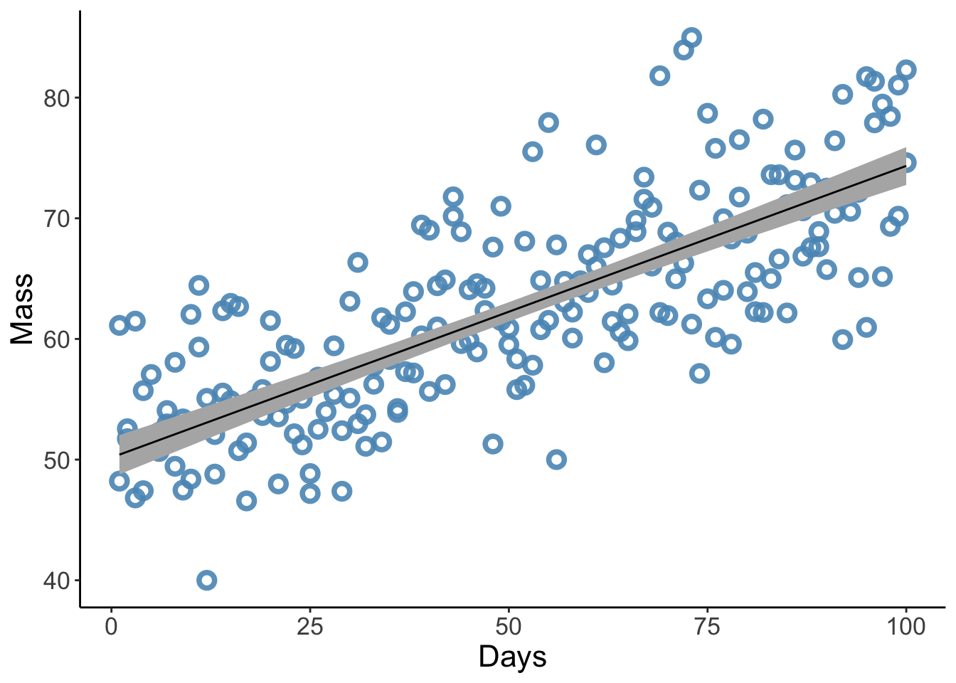
Let’s plot these

Code

p3 <-
  ggplot(data = sim_growth_data_small, 
         aes(x = Days)) +
  geom_point(aes(y = Mass),
             color = met.brewer(name = "Hokusai3")[4], shape = 1.5, stroke =2, size = 2.5, alpha = 0.9) +
  geom_smooth(data = Model_predictions,
              aes(y = Estimate, ymin = Q2.5, ymax = Q97.5),
              stat = "identity",
              fill = "grey70", color = "black", alpha = 1, size = 1/2) +
  labs(y = "Mass") +
  theme_classic() +
  #coord_cartesian(xlim = range(-4, 4),
  #               ylim = range(Kalahari_data$weight)) +
  theme(text = element_text(size = 16),
        panel.grid = element_blank())

p3

What if we wanted to plot the distribution of the intercept?

We could get the prediction from fitted when Days = 0 or we can use the as_draws_df function

Code

Our_mass_model_small %>% 
  as_draws_df()

# A draws_df: 2000 iterations, 4 chains, and 5 variables
   b_Intercept b_Days sigma lprior lp__
1           51   0.22   6.0   -9.6 -645
2           52   0.22   5.9   -9.5 -645
3           52   0.21   5.4   -9.0 -647
4           48   0.28   6.1   -9.7 -647
5           51   0.24   5.8   -9.5 -645
6           50   0.24   5.2   -8.7 -645
7           50   0.25   6.1   -9.7 -644
8           51   0.23   5.6   -9.3 -645
9           51   0.23   5.5   -9.1 -645
10          49   0.24   6.0   -9.5 -646
# ... with 7990 more draws
# ... hidden reserved variables {'.chain', '.iteration', '.draw'}

This gives us 2000 values for all the parameters estimated by the model - when plotted together these give us posterior distributions. Let’s do so for the Intercept.

Code

p4 <- 
  Our_mass_model_small %>% 
  as_draws_df() %>% 

  ggplot(aes(x = b_Intercept)) +
    stat_halfeye(fill = met.brewer("Hokusai3")[2], .width = c(0.66, 0.95), alpha = 1,
               point_interval = "mean_qi", point_fill = "white", 
               shape = 21, point_size = 4, stroke = 1.5, scale = 0.8) +
  labs(x= "Mass at day zero (the intercept)", y = NULL) +
  theme_classic() + 
  coord_cartesian(xlim = c(45, 55)) +
  theme(panel.background = element_rect(fill='transparent'), #transparent panel bg
        plot.background = element_rect(fill='transparent', color=NA), #transparent plot bg
        panel.grid.minor.x = element_blank(),
        legend.position = "none", #transparent legend panel
        text = element_text(size=16))

p4

Finally, we can combine the plot to make them look nice

Code

p3 + p4

\(~\)

Homework week 4

---

To get the data lets load rethinking

Code

library(rethinking)

data(Dinosaurs)

Dinosaur_data <- as_tibble(Dinosaurs) %>% 
  mutate(log_mass = log(mass))

Lets see what this data looks like

Code

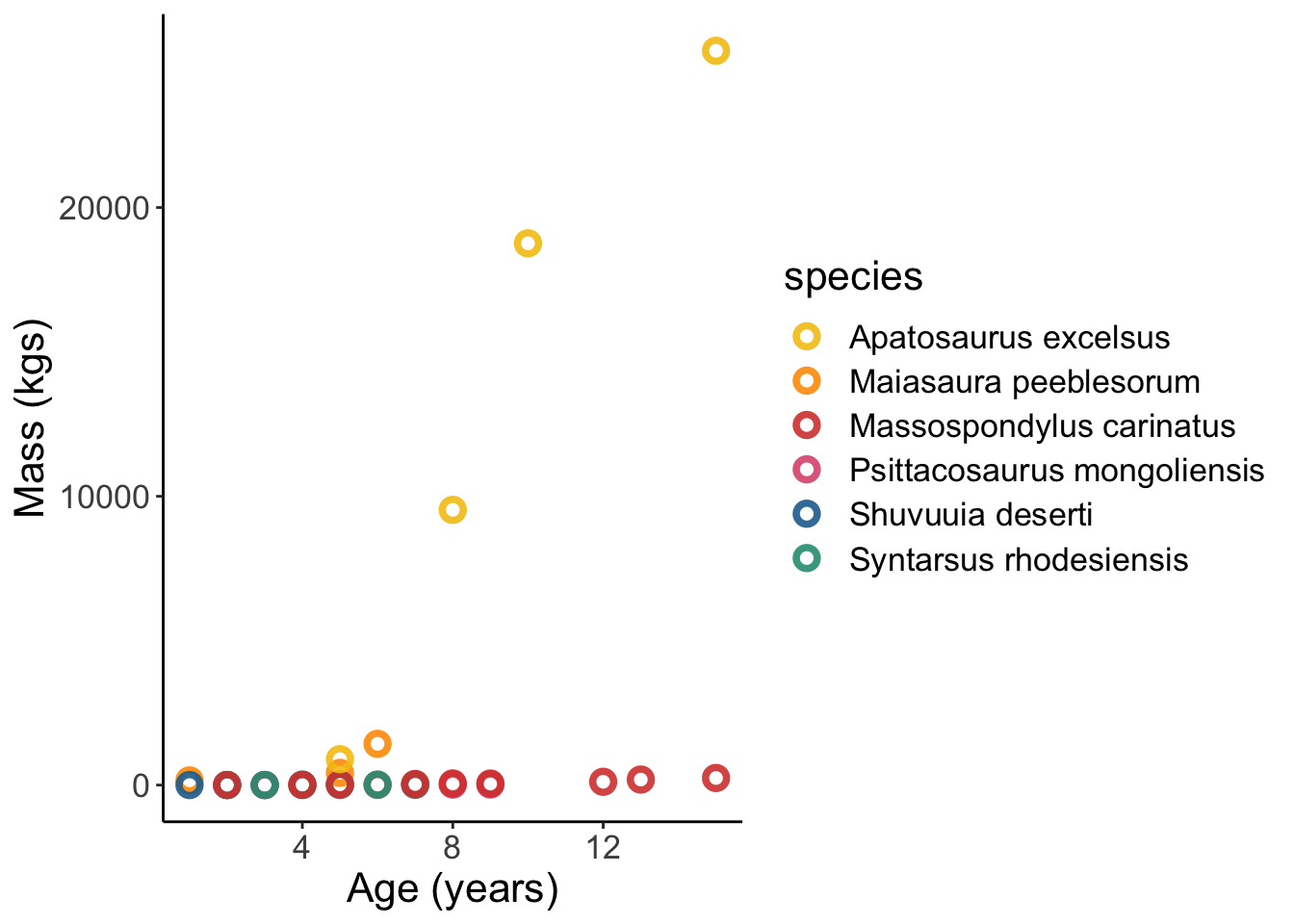
Dinosaur_data %>% 
  ggplot(aes(x = age, y = mass, colour = species)) +
  geom_point(shape = 1.5, stroke =2, size = 2.5, alpha = 0.9) +
  labs(x = "Age (years)", y = "Mass (kgs)") +
  scale_color_manual(values=met.brewer("Signac", 6)) +
  theme_classic() +
  theme(panel.grid = element_blank(),
        text = element_text(size = 16))

Ok this visualisation is no good because Apatosaurus is way off the charts. Lets log() the data.

Code

Dinosaur_data %>% 
  mutate(log_mass = log(mass)) %>% 
  ggplot(aes(x = age, y = log_mass, colour = species)) +
  geom_point(shape = 1.5, stroke =2, size = 2.5, alpha = 0.9) +
  labs(x = "Age (years)", y = "log(kgs)") +
  scale_color_manual(values=met.brewer("Signac", 6)) +
  theme_classic() +
  theme(panel.grid = element_blank(),
        text = element_text(size = 12))

Code

library(loo)

species_mass_model <- brm(data = Dinosaur_data,
    log_mass ~ 0 + species,
    family = gaussian,
    chains = 4, cores = 4, warmup = 1000, iter = 2000,
    file = "fits/species_mass_model")

species_mass_model <- add_criterion(species_mass_model, criterion = "waic")


species_mass_model_age <- update(species_mass_model,
                                 newdata = Dinosaur_data,
                                 formula = log_mass ~ 0 + species + age,
                                 file = "fits/species_mass_model_2")

species_mass_model_age <- add_criterion(species_mass_model_age, criterion = "waic")


species_mass_model_age_2 <- update(species_mass_model,
                                 newdata = Dinosaur_data,
                                 formula = log_mass ~ 0 + species + age + I(age^2),
                                 file = "fits/species_mass_model_3")

species_mass_model_age_2 <- add_criterion(species_mass_model_age_2, criterion = "waic")
  
  
  
species_3 <- update(species_mass_model,
                                 newdata = Dinosaur_data,
                                 formula = log_mass ~ 0 + age,
                                 file = "fits/species_mass_model_4")

species_3 <- add_criterion(species_3, criterion = "waic")

loo <- loo_compare(species_mass_model, species_mass_model_age, species_mass_model_age_2, species_3, criterion = "waic")

print(loo, summary = F)

                         elpd_diff se_diff
species_mass_model_age_2   0.0       0.0  
species_mass_model_age    -5.5       3.1  
species_mass_model       -33.0       4.0  
species_3                -50.5       4.0  

\(~\)

Homework week 5

---

Code

data(NWOGrants, package = "rethinking") # this loads WaffleDivorce as a dataframe without loading rehtinking

NWO_data <- 
  NWOGrants %>% 
  as_tibble()

Q1

These data are outcomes for scientific funding applications.

1a. Draw a DAG for the sample.

1b. Estimate the TOTAL causal effect of gender on grant awards

Lets fit the model

Code

model_template <- 
  brm(data = NWOGrants,
    family = binomial(),
    awards | trials(applications) ~ 1,
    prior = c(prior(normal(0, 1), class = Intercept)),
              #prior(normal(0, 1), class = b),
              #prior(exponential(1), class = sigma)),
    warmup = 1000, iter = 2000, chains = 4, cores = 4, 
    file = "fits/hw5_1")

total_effect <- 
  brm(data = NWOGrants,
    family = binomial(),
    awards | trials(applications) ~ 1,
    prior = c(prior(normal(0, 1), class = Intercept)),
              #prior(normal(0, 1), class = b),
              #prior(exponential(1), class = sigma)),
    warmup = 1000, iter = 2000, chains = 4, cores = 4)

Q2

Estimate the direct effect now